The following notes were written during the Covid ‘lockdown’ when there was much use of the term “exponential growth” – typically incorrectly. Besides, the occasional ‘cute’ picture does no harm!

Exponential growth has been much in the news recently. A
common example to illustrate exponential growth is the rabbit. As a
simple (and rather inaccurate) model assume each pair (best to work in
pairs, here) of rabbits can raise 20 kittens (that's the proper name)
in a year. Assume they do this for only one year: the numbers
are approximately right. This implies that the rabbit
population can increase by a factor of 10 every year.
(Actually it could be up to double this,
hence the
expression ...)
A rabbit weighs about 1.5 kg. The Earth weighs
6×1024 kg or
4×1024 rabbits.
Thus rabbits could consume the planet in about 24 years, give or take
a month or two.
This has not happened. There are limits to exponential growth.
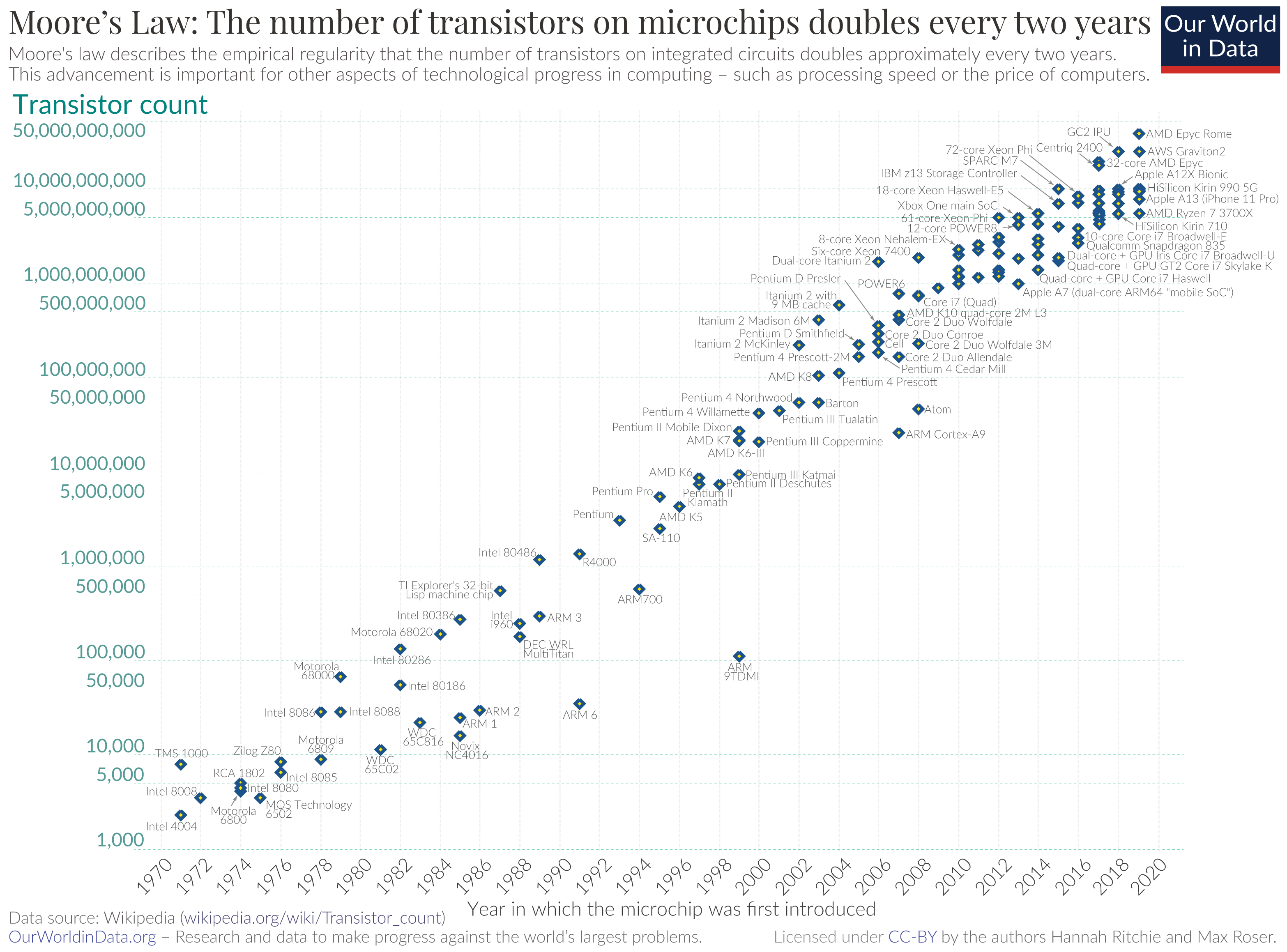
The so called “Moore's Law” observes the exponential growth in the number of components on an integrated circuit doubling every 18 months which has more-or-less held for over 50 years. There's a short (2 min.) video from Intel which says this!
In this time the rabbits might have consumed the whole galaxy.
Most of the progress in computing has resulted from the scaling of components. The ‘leading edge’ production processes had a ‘feature size’ of 10 μm in 1971 which had shrunk to 5 nm by 2021. Components are laid out on a 2D surface so that is (more or less) 20002 = 4 million times as many parts. A 2021 System on Chip (SoC) may be typified by the Apple A14 with over 1010 transistors for portable computing.
Further reading: this article is clear and short, if a little dated now (2012).
Like the rabbits, this will not (cannot!) continue indefinitely however it has continued for a surprisingly long time, partly because the technologists have come to expect it and, therefore invest in making it true.
All atoms are roughly an angstrom (1 Å) across (Si radius 1.11 Å). An angstrom is 0.1 nm. Thus structures are now tens of atoms across and the shrinking cannot continue much longer!
We're all familiar with Moore's Law and some of its consequences. In this module we look at the implications of the technology scaling and the architectural implications.
Reducing component size broadly results in:
Before concluding this introduction, there needs to be a mention of Dennard scaling which observed that the power consumption of chips stayed roughly constant as their density and speed increased. Unfortunately this is no longer true and power has become a dominating factor in SoCs. Power matters because:
As an analogy to the memory wall, there is also a “power wall”. This module does not delve deeply into this: sufficient to say that power management is an increasing concern. In high performance devices it is necessary to ration power by keeping some subsystems switched off at any given time: this is referred to as “dark silicon” - which also sounds cool!
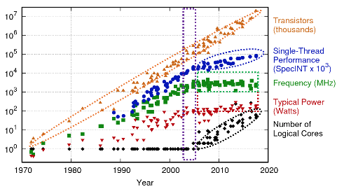
For further ‘reading’ you might try this slide show (16 mins. as a video/30 slides). The video version is a bit ... robotic ... and not all of it might make sense at this moment. It shows some trends and may be better flip through the slides and revisit it later in the semester.
Crudely, the Amdahl/Case Law suggests that a ‘balanced’ computer system needs about 1 megabyte of memory and 1 megabit/s of I/O per MIPS of CPU performance.
A contemporary desktop computer might have a quad-core processor, each core maybe sustaining two instructions per clock and a 3 GHz clock rate - so about 24,000 MIPS and, maybe, 16 GiB of RAM; according to that ‘law’, about right!
An early (1980s) home computer could achieve around 0.5 MIPS in real terms - although these were 8-bit operations so several would be needed for any ‘real’ calculation - and, maybe, 32 KiB of RAM; so roughly in balance.
A major issue to note in the evolution over this time is that the processors and memory have scaled differently.
In those early microprocessor systems the main memory speed was about twice that wanted by the processor. Memory ‘speed’ has increased by about 7%/year. Processor demands have increased by about 60%/year. These memories are now up to 10× faster whereas processors are over 1000× faster. The disparity in these speeds is known as the “memory wall”.
Here's a 2 min. video with someone sketching some plots.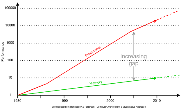
There are two important metrics:
With respect to processor ‘speed’, historically much of the increase resulted from faster circuits. Now it comes from primarily from increasing parallelism, both at the instruction level and by having multiple processors. Some of this parallelism can be employed by the hardware with single threaded code. However there is a rapidly increasing demand for multi-threaded software if the full benefits are to be exploited.
What is the speed of light?
3 ×10⁸ m.s-1
... and now in more appropriate units:
one foot (30 cm) per nanosecond.
(This is in a vacuum: the electrical signal propagation speed will be
somewhat slower but still quite similar.)
Remember a period of 1 ns correponds to a frequency of 1 GHz.
This is another barrier to performance. The most noticeable
consequence is probably the need to ‘balance’ the delays
on PCB (Printed Circuit Board) tracks, commonly visible on memory
buses. You may be able to see this on your PC motherboard where
tracks may be artificially lengthened to match those which have to be
longer.
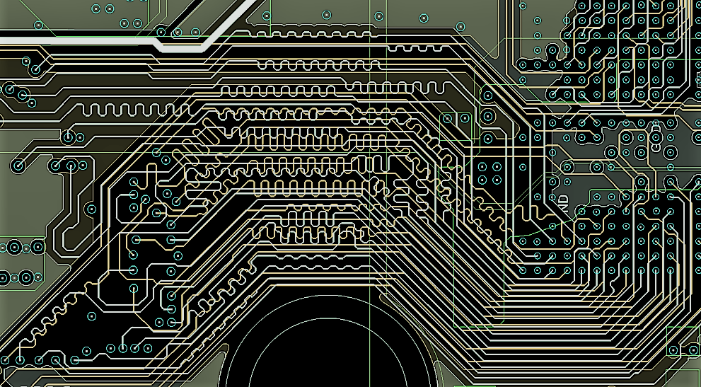
Click on image for full article and attribution.
Another consequence is the distance on a silicon chip. At frequencies
of (say) 3 GHz a signal cannot cross a large chip within a clock
cycle. This causes designers to subdivide a chip into smaller timing
regions. Single buses are impractical at such speeds and there
is an increasing tendency to employ Network on Chip (NoC) for
interconnection.
The latency and bandwidth restrictions off chip are, of course,
much more challenging.
Next: addressing.