Caches accelerate memory access. Another way of expressing this is thinking cache misses impose a performance penalty.
Every memory access can be thought of as one cycle plus a further
penalty for each access which is discovered to miss.
Average cycle time = 1 + miss rate × miss penalty
Thus if the penalty is high the performance will be significantly impaired if the miss rate is also high. Contemporary main memory will typically be at least 100× slower than the processor.
Note that ‘miss rate’ is more frequently quoted than ‘hit rate’, since hit rates are often values around 99.9%, 99.8%, 99.5% etc. which sound more similar than their effects actually prove.
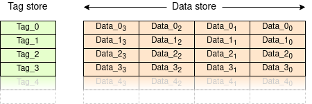
Any cache can be subdivided into two main components:
There may also be data such as validity which indicates if the copy is there or not.
Many caches exploit spatial locality by sharing a single tag across a block of adjacent addresses; this saves storing lots of tags when they would typically have repeated values. This block is known as a ‘cache line’.
There are various different names used for cache architectures but basically there are two approaches: high associativity and low associativity. It's easiest to introduce caches which are fully associative first.
Let's save space on this page by working with a 16-bit space: the
principle extends as needed. We'll assume four words per line as in
the figure above. Plus, we'll work in hexadecimal (what else?).
Start with an empty cache: all the lines are marked as invalid.
Decide to cache a memory word
(say,
Fill the chosen line with data from across the aligned
addresses: i.e. {
Repeat this process each time another line should be cached.
When checking the cache, the input address (with the lower bits separated) is checked against all the valid tags in the hope that one will match. There's actually a good chance and, if it does, the (few) remaining address bits select the word or byte from the line.
This is what is described above. Any data element can be cached in any of the cache locations. It is the most flexible architecture and, for a given size, will give the best hit rate. The problem is that the input address needs to be compared with all the tags on every access, which is expensive, especially in energy. It can also be slow because (practically) reading the data has to wait until the correct tag is determined.
This is the opposite extreme. There is only one place any given element can be cached. To extend the example above,
{
Assuming, for illustrative purposes, a not-too-big cache, addresses
This makes ‘choosing’ where to put a fetched line trivial (there is no choice!). It restricts the cache flexibility so it lowers the hit rate. On the other hand it makes a cache look-up much easier since the address being checked only needs to be compared with one entry whose position is known from the incoming address. This saves a lot of energy. It also offers the chance to speed up access since the data read is typically done speculatively, in parallel with the tag comparison in the hope that it will be a hit. In many circumstances a hit is confirmed and the data is already ready to return.
Direct mapped caches can suffer quite badly from conflicts if the application is unlucky. To alleviate this, set associative caches offer a bit more choice. A ‘two-way’ set associative cache is basically two direct mapped caches in parallel, thus offering two possible places any datum may be cached and preventing some conflicts. The sets will each be half the size, of course.
A four-way set associative cache will have four, quarter size sets etc.
A set associative cache will usually have a better hit rate than a direct mapped cache, but worse than a fully associative cache, of the same total capacity. Similarly its energy requirements will be in between the extremes.
The tool below allows a comparison of different cache
architectures. The scale diagram is accurate in the logical
representation of the cache: the physical layout will sometimes
differ. The statistics show the overheads and how the memories are
organised. An important aspect is that low-order bits are used
‘directly’ to exploit spatial locality and the tags are
the high-order address bits.
Particular points to notice are:
The areas in the set diagram (on the left) are scaled to the panel size. The relative proportions (widths) of the tag and data areas are to scale.
The areas in the layout (right hand) figure are to scale
with (addressed) lines spread vertically and data indicated
horizontally.
(The data multiplexer, when present, is exaggerated
so it can be seen.)
The physical layout on the chip will be
‘squarer’ than most of these examples.
The figure can show the cost of a cache architecture in terms of area and power. The effectiveness of the cache is determined by its hit rate which itself is heavily influenced by the behaviour of the code it is running. It is therefore not possible to represent this here. In general the hit rate will be increased as the size and associativity increase and be (slightly) decreased as the line length increases.
Puzzle: Why is the tag overhead (significantly) greater in a 64-bit architecture rather than a 32-bit architecture with the same size cache?
Low associativity is simpler, and faster and lower power when the cache hits but will have more misses which are slow and power hungry. For most real access patterns the hit rates of all are quite high. If a cache is large then associativity will make quite a small difference to the hit rate and low associativity will be preferred. On the other hand, in a small cache, high associativity will provide a noticeable advantage.
The outcome also depends on the access patterns of course. With a direct mapped cache a single conflict could have serious consequences for performance. Consider two, frequently used procedures which are called alternately. If their code addresses conflict they can cause ‘thrashing’ where they keep displacing each other, sacrificing any advantage. A minor edit to the code could cause such a circumstance to appear or disappear and this would be mysterious for most programmers! More sets do not eliminate such issues but do make them much less likely.
In a cache hierarchy it is possible that the level 1 cache might have 4- or 8-way associativity whereas the level 3 cache could be direct mapped. Full associativity is rare in such caches nowadays since even level 1 caches are usually quite sizeable. Full associativity may be used in other structures such as MMUs, branch predictors etc.
In operation an incoming address (from a load, store or instruction
fetch) is logically divided up into the fields as coloured in the
example above. In a direct mapped cache one line is selected with the
low-order bits (red). In a set associative cache the same thing
happens but in each set.
The chosen line(s), tag and data are read. This incoming tag bits
(green) are compared with the read tag(s). If there is no match then
the cache has missed. If there is a match then the cache has
hit.
More on what happens on a cache miss later.
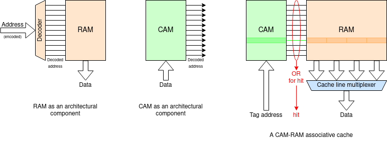
A fully associative cache works in the same way, but because it has (in principle) to read and compare every cache entry it is usually implemented differently. To avoid reading everything each time (expensive!) there may be a two-stage process (slower) with the comparison may be done using a CAM; this indicates a hit line which is fed to read a subsequent RAM.
You've met RAM before (we hope!).
When a RAM is read an address is fed in (being decoded to a
‘one hot’ code on the way) and a data pattern is read out
from that location.
A CAM is like the same block, working in reverse: a data pattern is
fed in and the address at which it is found comes out ... assuming
that the address was present. We won't go into it
in
detail here.
CAM is also known as "associative store"; the reason should be
clear.
It perhaps should be emphasised that the cache
‘search’ is a parallel operation, independent of the
number of entries searched. Contrast this with software searching a
table where it would need to iterate and the search time would depend
on the table size.
Another (common) use of CAM is recognising patterns in network routeing*.
* I still prefer the English spelling.
In the example below there is an 8 location cache for a
64 location memory. The highlighted address bits index
which line (in each set, if appropriate) locations can be cached; the
non-highlighted bits (there would be more in a real scale example)
would be the tag. The lines in the memory (right) are coloured to
correspond. Each set in the cache can contain, at most, one
line in each colour.
The extreme right strip represents the selection of lines in current
use – the ‘working set’. (This starts with
an arbitrary choice, with a few blocks of adjacent lines, somewhat
reminiscent of the patterns used in typical software. These would be
OS-organised ‘segments’, for the object code, global
variables, stack etc.)
The intention is to illustrate that, for a realistic working set, the best cache utilisation (fewest empty lines) is typically achieved when the set index is taken from the least significant bits, interleaving the cache lines (different colours) to the maximum extent. This can be seen by altering the bit choice and looking, particularly, at the total of unused lines. With the initial working set this can be seen in most, but not all of the settings.
Typical working sets will comprise a few blocks of
contiguous addresses. A representative sample in this example might
be 10-20 addresses in total: an example has been
preloaded.
Higher associativity usually improves utilisation; the extra freedom
can't make it worse. It will have a penalty in speed and (cache)
power though - particularly at very high associativity.
Generally, better occupancy is achieved by choosing less
significant address bits to index the sets. This is particularly
noticeable at low associativity.
Next: more about caches.